The following are some examples of how to set up OPS variables to cross reference signal tag data from a SCADA system.
Example 1: Average DO for the day
We want to capture the average DO for the day; this is a sample of our data and how to setup the OPS variable:
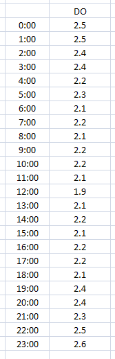
We have 24 data points that total 54.2. Our average DO for the day will be 2.258333 (depending on number of decimal places set for this variable). The value is stored on the start day and time.
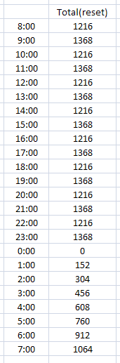
Example 2: Average DO from 8 AM to 8 AM the next day
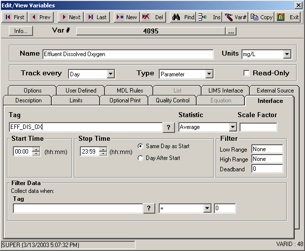
In this example we need the average DO but we want to start and end the readings at 8 AM. Here is a sample of data and how to set up the variable in OPS.

The number of data points is 24 again, and the total is 54.2, so our average will be the same as example 1 = 2.258333. Notice we selected Day After Start. This tells OPS that the Stop Time is the day after the Start Time. The value is always stored on the start day and time.
If you set these times and left Same Day as Start, OPS would think you wanted data from 7:59AM to 8:00AM of the same day – what is the average for one minute of the day – which is wrong!
By setting Day After Start, OPS knows you want the average DO from 8 AM on one day to 7:59 AM the next day.
Example 3: Total flow from a daily totalizer that resets at midnight.
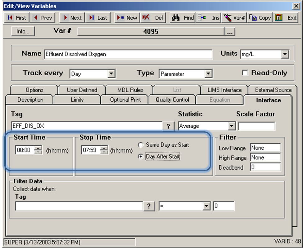
“Total flow” can mean so many things, so it is important to know what flow you are talking about. A smart man told me, “think of a totalizer as an odometer – always counting up”. Now some totalizer meters always reset at midnight. This is how to set up an OPS variable to handle a flow totalizer that resets at midnight.
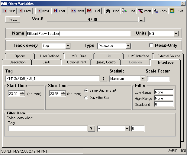
The value we will capture will be the highest number by midnight, which is 1368. Note: Why don’t we use last? In the case above, LAST would work, but if the SCADA system is logging data a fraction of a minute and the meter resets before 23:59 – you could end up with a reading of zero or something totally wrong!
Example 4: Total flow from a totalizer that doesn’t reset every day. (DIFF)
In the case of a totalizer that resets, but not every day, we need to use a different statistic – DIFF. This statistic calculates the difference between the first value and the last value for the period requested (i.e., if the variable is defined as an hourly variable, DIFF will get the first and last values for each hour and subtract them).
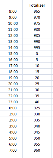
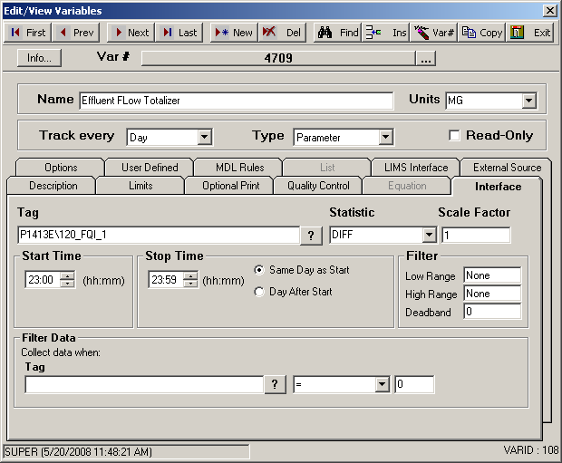
In our example, we have a daily variable that uses the default start and stop times. The midnight reading is 925 and the 23:59 reading is 40. We can see that the meter rolled over at 15:00 or 3 PM. We can see that the meter is approaching 999 which is the assumed rollover point in this example.
The interface will subtract the last value from the first, and if the result is negative then we have a rollover. By using logarithmic functions, we can determine that the rollover is 1000 and subtract the sum of the first and last readings. If there is no rollover, the interface simply returns the difference between the last value and the first value.
In our case, the difference of the last and first values is -885. The interface determines 1000 as the rollover by taking 10 to the power of the log of the number rounded up. Log of 885 is 2.9, rounded up to 3 and 10 to the power of 3 = 1000. It then subtracts the rollover from the first reading and then adds the last reading = 1000 – 925 + 40, giving us 115.
In our data we stepped the value by 5 every time, so 5 times 23 data point changes = 115.
Example 5: Total flow from an instantaneous flow meter reading
We’ve talked about totalizers as being like odometers; the next type of flow is like a speedometer and is called an instantaneous flow meter. This is a meter that might show how many gallons per minute (GPM) are flowing through a pipe, for example. We need to convert gallons per minute to millions of gallons per day (MGD). There are 1440 minutes in a day and we want one millionth of that number. So our Scale Factor will be 1440 / 1,000,000 or 0.00144. The following is some sample data and a screen of an OPS variable for this purpose:
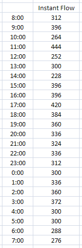
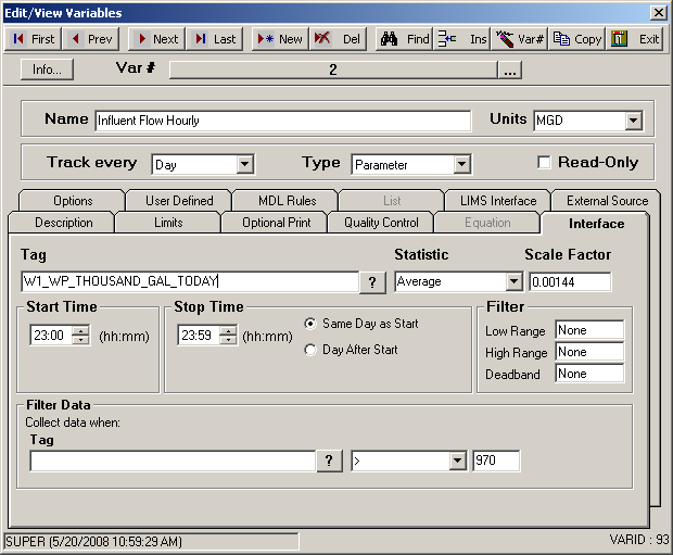
The average of GPM coming through the pipe is 333. When we convert the average by our Scale Factor of .00144 we get 0.47952 MGD. This is almost one half of one million gallons per day.
Why did we use Average instead of Total? We could have simply totaled the numbers and divided by the number of data points. In this case our total would be 7992. In order to calculate MGD, OPS would have to know how many data points were used to total 7992, because we still need the average flow. OPS SQL does not know this number and the number of data points could change from minutely to secondly values.
Example 6: Total flow from a tag that holds yesterdays (previous) total flow.
This peculiar tag holds the total flow from yesterday (or “previous” day). Typically it changes right after midnight to hold the new previous day. This is our sample data and how we set it up in OPS:
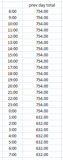
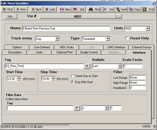
We see our value stays the same until after the midnight it changes to 632. We span over two days by setting the Start Time to 11 PM, Stop Time to 3 AM and select Day After Start. The value 632 will be stored at the start day and time. Why did we span the time so far apart? Keep in mind that Daylight Savings Time will affect your data twice a year so the cushion will mean we won’t have to worry about that.
Example 7: Get the average turbidity when BACKEB00 = 1.
The following examples use Filter and Filter Data. The difference is Filter will filter data value for a tag based on its own value. Filter Data will filter data value for a tag based on the value of a different tag.
The Filter controls are on the far right side of the Interface tab and the Filter Data controls are on the bottom of the Interface tab.
This first example shows how to filter turbidity values when BACKEB00 equals a value of 1. BACKEB00 could be analog data that changes constantly throughout the day or it can be a digital reading that just switches from 0 to 1 like when a valve opens and closes.
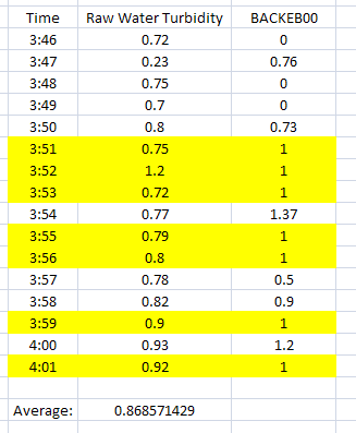
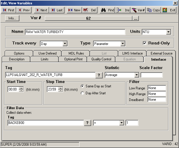
Notice that the average for the range of data we have selected only uses the values highlighted. BACKEB00 must be exactly one (1) because that is what we specified in the Filter Data.
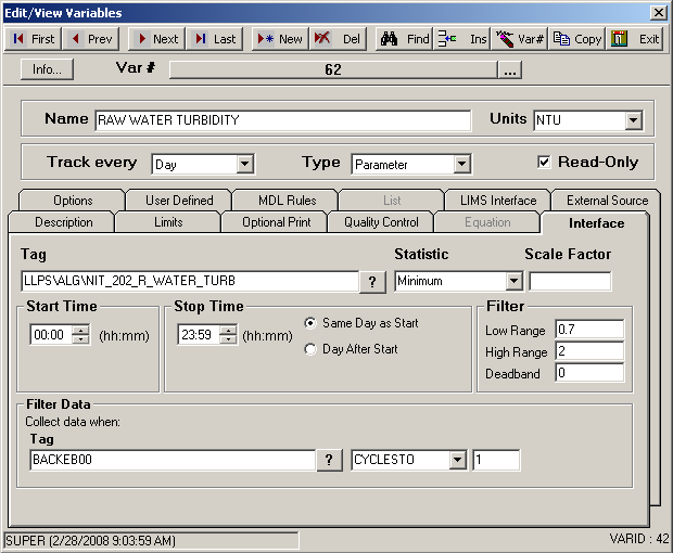
Example 8: Get the First reading when BACKEB00 changes to 1.
In this example we entered the text CYCLESTO in place of the equal sign (=) under Filter Data. In this example, we want to get the first value of turbidity when BACKEB00 changes to one (1) from any other value.
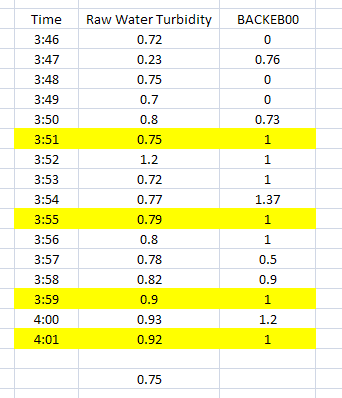

The example above shows all values highlighted that are applicable to this particular set up. Since our Statistic is First, the value returned from our sample data would be 0.75.
Example 9: Get the First reading 2 minutes after BACKEB00 changes to 1.
In this example we entered the text ACT(2) in place of the CYCLESTO. ACT stands for “After (tag) Cycles To” the value, which we set to a one (1). The (2) means two minutes. So when we put the two items together we get ACT(2) = After (tag) Cycles To a 1, get the value two minutes later, or “Get the value two minutes after the tag cycles to one.”
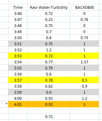

The rows highlighted in grey are when BACKEB00 cycles to 1, and the yellow highlighted rows are two minutes later. Notice that at 4:01 both apply, it has cycled to 1 and it is a value two minutes after a cycle to 1 occurrence. One does not negate the other. Since our Statistic is First, our returned value will be 0.72.
Example 10: Get the Minimum greater than 0.7 but no higher than 2.0.
We are expecting turbidity readings between 0.7 and 2.0. Anything else is either a false reading to us or we just don’t want values outside that range. The following example shows how we set that up to get the minimum reading above 0.7.
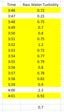
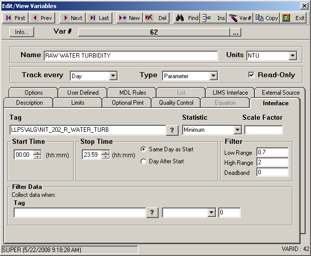
Almost all the rows are highlighted this time, except for the two that are out of our range. Notice how we set up the Filter controls on the far right of the Interface tab. Since our Statistic is Minimum this time, our value returned will be 0.7. The Low Range filter will look for values equal to or higher and the High Range looks for values equal to or less than. When both conditions are used as shown above, They both apply simultaneously.
Example 11: Get the Minimum greater than 0.7 when BACKEOO CyclesTo 1.
Now let’s look at an example that uses all parts. We want to get the lowest turbidity reading that is between 0.7 and 2 but only when BACKEB00 cycles to a one (1).
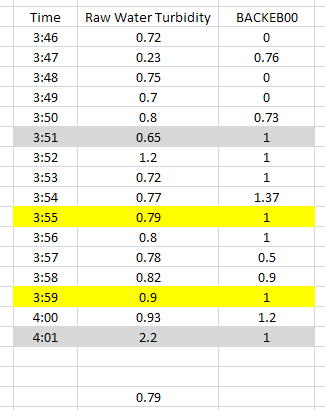
In our data, BACKEB00 cycles to 1 four times but only two fall within the Filter ranges. Since our Statistic is Minimum, our value will be 0.79.